Single Variable Linear Regression

Linear Model and Residual Assumption

Single variable linear regression models a response variable $y$ as a linear function of a regressor variable $x$ plus a random component.

\[y=\beta_0+\beta_1 x+\epsilon\]

For each observation of the variables $i$:

\[y_i=\beta_0+\beta_1 x_i+\epsilon_i\]

The essential assumption in linear regression is that the random component draws from a distribution that is identical for all observations $i$. This distribution is Normal with mean $0$ and some true variance $\sigma^2$.

Assumption: $\epsilon_i \sim N(0, \sigma^2) \, \forall i$

Since $\mathbb{E}[\epsilon_i]=0$ the prediction $\hat{y}$ from the linear model is:

\[\hat{y}_i = \mathbb{E}[y | x=x_i]=\beta_0+\beta_1 x_i\]

The difference between the true $y$ value and predicted $y$ value is the residual $e_i=y_i-\hat{y}_i$.

Under the assumption, each residual $e_i$ samples from idependent and identically distributed Normal random variables. The residuals should not only have mean zero, but also have the same variance over all $x,y$.

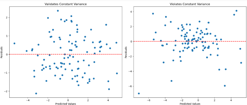
This assumption can be visually verified by a residual plot. If the residuals do not appear to have constant variance, then the underlying model of the data is unlikely to be linear. However, a linear model could still be a useful approximation for data within a certain range of values.

For example, the left plot shows residuals from a dataset that likely follows a true linear model. The right plot shows residuals that change over different $y$ values so the underlying data distribution is unlikely to be linear. However, in the middle of the $y$ range, the linear model is fairly accurate.

Least Squares Estimation

Linear regression is the method of estimating $\beta_0, \beta_1$ in a linear model from a known dataset. Linear regression is uses ordinary least squares estimation (abbreviated LS, OLS, LSE), meaning that its objective is to minimize the sum of squared residuals.

\[\hat{\beta}_0, \hat{\beta}_1 = \underset{\beta_0, \beta_1}{\operatorname{argmin}} L(\beta_0, \beta_1)\] \[L(\beta_0, \beta_1) = SSE = \sum_{i=1}^n\left(y_i-\hat{y}_i\right)^2=\sum_{i=1}^n\left(y_i-\beta_0-\beta_1 x_i\right)^2\]

The objective is called a loss function since it represents error. The loss function for linear regression, sum of squared error, is a convex function with respect to $\beta_0, \beta_1$ so the single global minimum can be found by taking the first derivative and setting it equal to zero.

\(\frac{\partial L}{\partial \beta_0}=-2 \sum_{i=1}^n\left(y_i-\beta_0-\beta_1 x_i\right)\) \(\frac{\partial L}{\partial \beta_1}=-2 \sum_{i=1}^n\left(y_i-\beta_0-\beta_1 x_i\right) x_i\)

\[\left\{\begin{array}{l} -2 \sum_{i=1}^n\left(y_i-\hat{\beta}_0-\hat{\beta}_1 x_i\right)=0 \\ -2 \sum_{i=1}^n\left(y_i-\hat{\beta}_0-\hat{\beta}_1 x_i\right) x_i=0 \end{array}\right.\]

The first equation can easily be rearranged to isolate \(\hat{\beta}_0\) by distributing the summation.

\[-2 (\sum_{i=1}^ny_i- n \hat{\beta}_0-\hat{\beta}_1 \sum_{i=1}^n x_i)=0\] \[\hat{\beta}_0 = \frac{1}{n} \sum_{i=1}^ny_i -\hat{\beta}_1 \frac{1}{n} \sum_{i=1}^n x_i\]

The algebra to substitute this into the second equation is a little long so let’s skip to the solution for \(\hat{\beta}_1\) and express it using shorthand notation. Let $\bar{x}=\frac{1}{n} \sum_{i=1}^n x_i$ be the sample mean of $x$ in the known dataset and $\bar{y}=\frac{1}{n} \sum_{i=1}^n y_i$ be the sample mean of $y$. Now let’s define the “sum of squares” or “sum of deviations” xx, xy, and yy.

\[\begin{aligned} & S_{x x}=\sum_{i=1}^n\left(x_i-\bar{x}\right)^2=\sum_{i=1}^n x_i^2-\frac{1}{n}\left(\sum_{i=1}^n x_i\right)^2 \\ & S_{xy}=\sum_{i=1}^n\left(x_i-\bar{x}\right)\left(y_i-\bar{y}\right)=\sum_{i=1}^n x_i y_i-\frac{1}{n} \sum_{i=1}^n x_i \sum_{i=1}^n y_i \\ & S_{yy}=\sum_{i=1}^n\left(y_i-\bar{y}\right)^2=\sum_{i=1}^n y_i^2-\frac{1}{n}\left(\sum_{i=1}^n y_i\right)^2 \\ \end{aligned}\]

The solution is then

\[\hat{\beta}_1=\frac{S_{x y}}{S_{x x}} \quad \hat{\beta}_0 = \bar{y}-\hat{\beta}_1 \bar{x}\]

With the notation above, complete knowledge of the dataset is not necessary. All the values can be calculated from the number of datapoints $n$, sums $\sum_i x_i, \sum_i y_i$, sums of squares $\sum_i x_i^2, \sum_i y_i^2$, and dot product $\sum_i x_iy_i$.

Example

A gas station has recorded the daily demand in gallons at 100 different prices. Linear regression can model demand as a function of price. The dataset is 100 rows and 2 columns with one column $p$ for historical price and $d$ for observed demand. The dataset produces the following calculations:

\[\begin{aligned} & \sum_i p_i=348.5, \sum_i d_i=1011.7, \\ & \sum_i p_i^2=1289.5, \sum_i d_i^2=12406.0, \\ & \sum_i p_id_i = 3141.0 \end{aligned}\] \[\hat{\beta}_1=\frac{S_{x y}}{S_{x x}} = \frac{3141.0 - 348.5 \cdot 1011.7 / 100}{1289.5 - (348.5)^2 / 100} = -5.132\] \[\hat{\beta}_0 = \bar{y}-\hat{\beta}_1 \bar{x} = 1011.7 / 100 - (-5.132) (348.5) / 100 = 28.002\]

The linear model is: $\hat{d}_i = 28.002 - 5.132 p_i $

All other values associated with linear regression can also be found from these calculations. For example, using the formula dicussed later:

\[R^2=\frac{S_{x y}^2}{S_{xx} S_{y y}} =\frac{(3141.0-(348.5)(1011.7)/100)^2}{(1289.5-(348.5)^2/100)(12406.0-(1011.7)^2/100)}=0.910\]

The data somewhat closely follows the linear model. I generated the dataset using a linear model with a large random term.

import numpy as np
p = np.linspace(2, 4.97, 100)
d = 25 - 5 * p + 5 * np.random.rand(100)
print(np.sum(p), np.sum(d), np.sum(p**2), np.sum(d**2), np.sum(p*d))

ANOVA: Significance of Model

Analysis of Variance (ANOVA) is a technique to determine whether the linear model is statistically significant. If a model is statistically significant, that means that under the assumption that the dataset is accurate, the variability and size of the dataset suggest that the estimated parameters \(\hat{\beta}\) are accurate with high confidence.

ANOVA is represented in a table with slightly different notation. Single-variable ANOVA looks at three sum of squares: regression, error, and total. Sum of squares regression measures the variation in $y$ explained by the regression. \(SSR=\hat{\beta}_1 S_{xy} = \frac{S_{x y}^2}{S_{x x}}\) Sum of squares error is the sum of squared residuals, the objective of linear regression. \(SSE=\sum_{i=1}^n e_i^2\) Sum of squares total is the sum of squared deviation in the response. \(SST=S_{yy}\)

$SST$ is the total because $SSR+SSE=SST$. The fast way to compute $SSE$ is using this fact: $SSE=SST-SSR=S_{yy}-\frac{S_{x y}^2}{S_{x x}}$

The second column in the ANOVA table is degrees of freedom. The regressor provides $1$ degree of freedom and the total degrees of freedom is $n-1$ so the degrees of freedom for error are $(n-1)-1=n-2$. The third column is mean squares, which is the sum of squares divided by degrees of freedom. The last column is a single value for the ratio of the two mean squares.

	SS	df	MS	$F_0$
R	SSR	1	SSR/1	MSR/MSE
E	SSE	n-2	SSE/(n-2)
T	SST	n-1

The CDF of the $F$ distribution with degrees of freedom $(1,n-2)$ evaluated at the test statistic $F_0$ provides the p-value for the ANOVA test of significance.

\[\text{p-value}=F_{1, n-2}\left(F_0\right)\]

The p-value is the probability of observing the sample data (or sample data further from the null hypothesis) assuming the null hypothesis is true. The null hypothesis for ANOVA is that the model is not significant. Thus if the p-value is low, the sample data provides strong evidence to reject the null hypothesis and conclude that the model is significant.

p-values are not intended for comparing models; if one model has a lower p-value it is not necessarily a closer fit. The hypothesis test is binary, whether the model is significant or not. I will repeat: model significance means that the dataset provides confidence in the estimated paramters $\hat{\beta}$. If the least-squares linear model is not significant, then the dataset does not follow a linear model. Model significance does not verify the assumptions that (1) the sample dataset is accurate and (2) the residuals are identically distributed.

Coefficient of Determination

In even simpler terms than the p-value, the coefficient of determination (r-squared) suggests whether the data follows a linear model. $R^2$ is always between $0$ and $1$. A larger value means that the data more closely follows a linear model, so r-squared is a good metric to easily compare models.

Definition: \(R^2=1-\frac{S S E}{S S T}=1-\frac{\sum_{i=1}^n e_i^2}{S_{y y}} =1-\frac{\sum_{i=1}^n (y_i-\hat{y}_i)^2}{ \sum_{i=1}^n (y_i-\bar{y})^2}\)

Computation: \(R^2=1-\frac{S S E}{S S T}=1-\frac{S S T-S S R}{S S T}=\frac{S S R}{S S T} =\frac{S_{x y}^2 / S_{x x}}{S_{y y}}=\frac{S_{x y}^2}{S_{xx} S_{y y}} \\ =\frac{(\sum_{i=1}^n x_iy_i-\frac{1}{n}(\sum_{i=1}^n x_i)(\sum_{i=1}^n y_i)) ^2}{(\sum_{i=1}^n {x_i}^2-\frac{1}{n}(\sum_{i=1}^n {x_i})^2)(\sum_{i=1}^n {y_i}^2-\frac{1}{n}(\sum_{i=1}^n {y_i})^2)}\)

Significance of Coefficients

Recall the key assumption of linear regression is that the residuals $e_i$ have an identical and normal distribution $\epsilon_i \sim N\left(0, \sigma^2\right)$. The variance of the error $\epsilon$ is another representation of how close the dataset fits a linear model - lower variance means less error. Since the error is the only random component of the model, the variance of error is also the variance of the model predictions. The variance can be estimated from the sample dataset.

$\hat{\sigma}^2=MSE =\frac{S S E}{n-2}=\frac{S_{yy}-S_{x x}}{n-2}$

The estimated variance can be used to find the standard deviation of the estimated parameters $(\hat{\beta}_0, \hat{\beta}_1)$. Since this standard deviation represents error, it is called standard error $\operatorname{se}$.

\[\begin{aligned} & \operatorname{se}\left(\hat{\beta}_1\right)=\sqrt{\frac{\hat{\sigma}^2}{S_{x x}}} \\ & \operatorname{se}\left(\hat{\beta}_0\right)=\sqrt{\hat{\sigma}^2\left(\frac{1}{n}+\frac{\bar{x}^2}{S_{x x}}\right)} \end{aligned}\]

The standard error can be used for hypothesis tests and confidence intervals for the parameters $\beta_{j=0,1}$. Since the error is assumed to be normally distributed, its variance estimated from a sample follows a $t$ distribution and the degrees of freedom is $n-2$ as per the ANOVA table.

The most important hypothesis test is “signifance” - whether the coefficients are nonzero with $\alpha$ confidence.

\[H_0: \beta_j=0 \quad H_1: \beta_j \neq 0\]

critical value $t_{\alpha/2, n-2}$

test statistic $t_0=\frac{\hat{\beta}_j-0}{\operatorname{se}\left(\hat{\beta}_j\right)}$

rejection region $\lvert t_0 \rvert > t_{\alpha/2, n-2}$

Interval Predictions

In addition to predicting a single point for $\beta$, a confidence interval can be predicted. The general form of a $1-\alpha$ confidence interval is $[$ mean $\pm$ critical value $\cdot$ std $]$.

\[\beta_j \in\left[\hat{\beta}_j \pm t_{\alpha / 2, n-2} \operatorname{se}\left(\hat{\beta}_j\right)\right]\]

Subsequently, a confidence interval for the “mean response” and “prediction” at $x_i$ can be formed. The mean response assumes that the data follows the linear model with the chosen parameters $\beta$. The prediction interval instead lenghtens the interval to account the error of the model $\sigma^2$.

\[y_i \in\left[\hat{y}_i \pm t_{\alpha / 2, n-2} \sqrt{\hat{\sigma}^2\left(\frac{1}{n}+\frac{\left(x_i-\bar{x}\right)^2}{S_{xx}}\right)}\right]\] \[y_i \in\left[\hat{y}_i \pm t_{\alpha / 2, n-2} \sqrt{\hat{\sigma}^2\left(\frac{1}{n}+\frac{\left(x_i-\bar{x}\right)^2}{S_{xx}} + 1 \right)}\right]\]